Challenges
•
Indoor scene inference
◦
Task가 많기 때문에
◦
Task label을 얻는 것도 힘들고, 서로 유사한 task도 많다
Research question
Do visual tasks have a relationship, or are they unrelated?
•
최적의 source task 및 target task를 고를 수 있는 fully-computational한 방법을 제시
•
task structure 추론
◦
“structure” is a collection of computationally found relations specifying which tasks supply useful information to another, and by how much
Hypothesis
•
Task 간의 관계가 밝혀진다면,
•
Task 중 몇개만 full annotation, 나머지는 다른 task로부터 fine-tuning해서
•
task 전반을 잘 학습할 수 있지 않을까?
Goal
•
mapping from X to Y
•
computes an affinity matrix among tasks based on whether the solution for one task can be sufficiently easily read out of the representation trained for another task
•
computationally found directed hypergraph that captures the notion of task transferability over any given task dictionary.
Methods
Notations
•
task dictionary
◦
: set of tasks which we want solved (target)
◦
: set of tasks that can be trained (source)
Methods
•
input : 4 million images for indoor scene inference
◦
26 tasks
◦
training (120k), validation (16k), and test (17k) images
•
output : A hypergraph of tasks
•
Schematic overview
STEP 1 : task-specific modeling
•
fully supervised task-specific network for each task in S
•
encoder-decoder architecture homogeneous across all tasks
•
Encoder's architecture : a fully convolutional ResNet-50 without pooling, identical across all task-specific networks
•
Decoder's architecture : depend on the task as the output structures of different tasks vary
•
Task-specific networks are trained on the training set
STEP 2: Train transfer functions among tasks
•
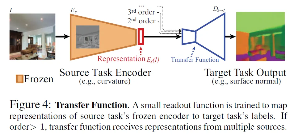
Transfer network from to
•
Learns readout function
◦
: ground truth of for image
•
Transfer’s architecture: identical shallow networks with 2 conv layers (concatenated channel-wise if higher-order
•
Transfer networks are trained on a subset of validation set, ranging from 1k images to 16k, in order to model the transfer patterns under different data regimes
High-order transfers
•
Same as first order but receive multiple representations in the input
•
e.g.)
•
a sampling procedure with the goal of filtering out higher-order transfers that are less likely to yield good results, without training them: a beam search
Beam search
Transfer results
STEP 3: Get task affinities
•
Derived from Analytic Hierarchy Process
•
구하기
◦
For each , we construct a pairwise tournament matrix between all feasible sources for transferring to
◦
의 값: tournament ratio: D_test에서 가 보다 transfer를 잘 한 images의 비율
•
: Normalize
•
We quantify the final transferability of to as the corresponding () component of the principal eigenvector of (normalized to sum to 1)
STEP 4: Compute global taxonomy
•
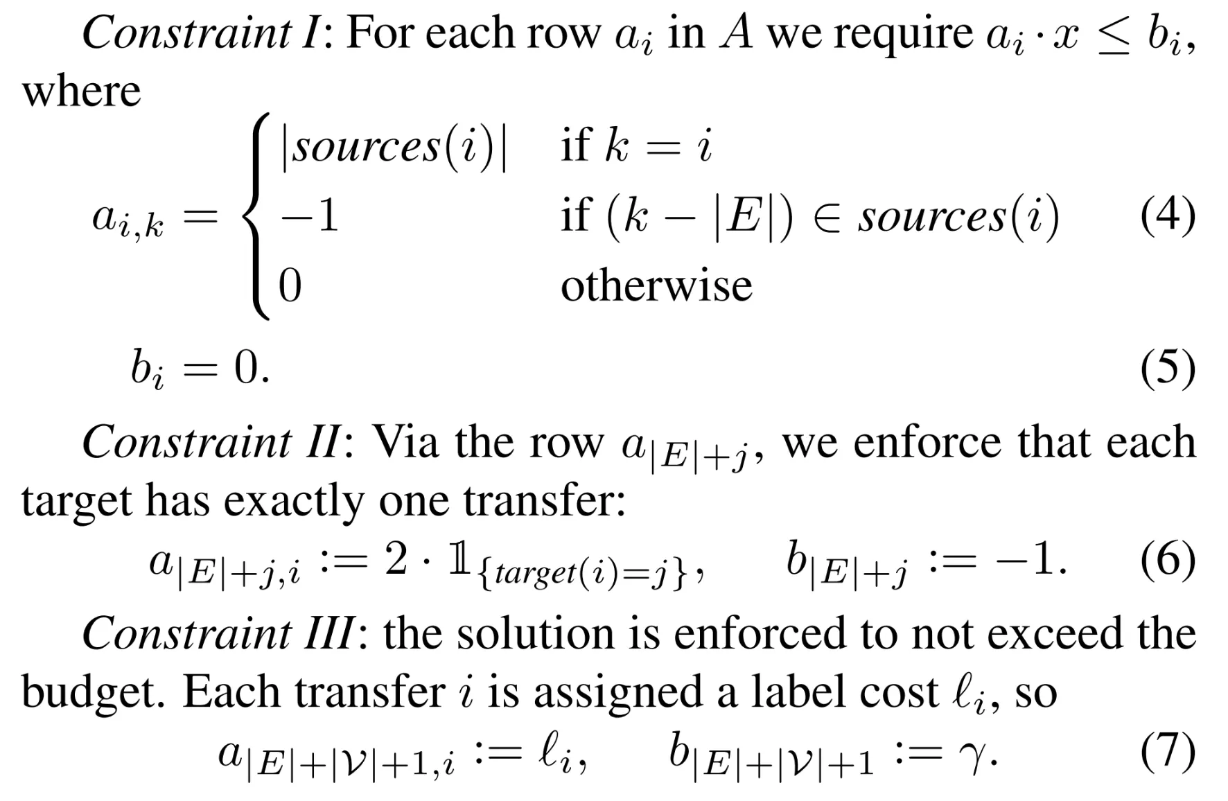
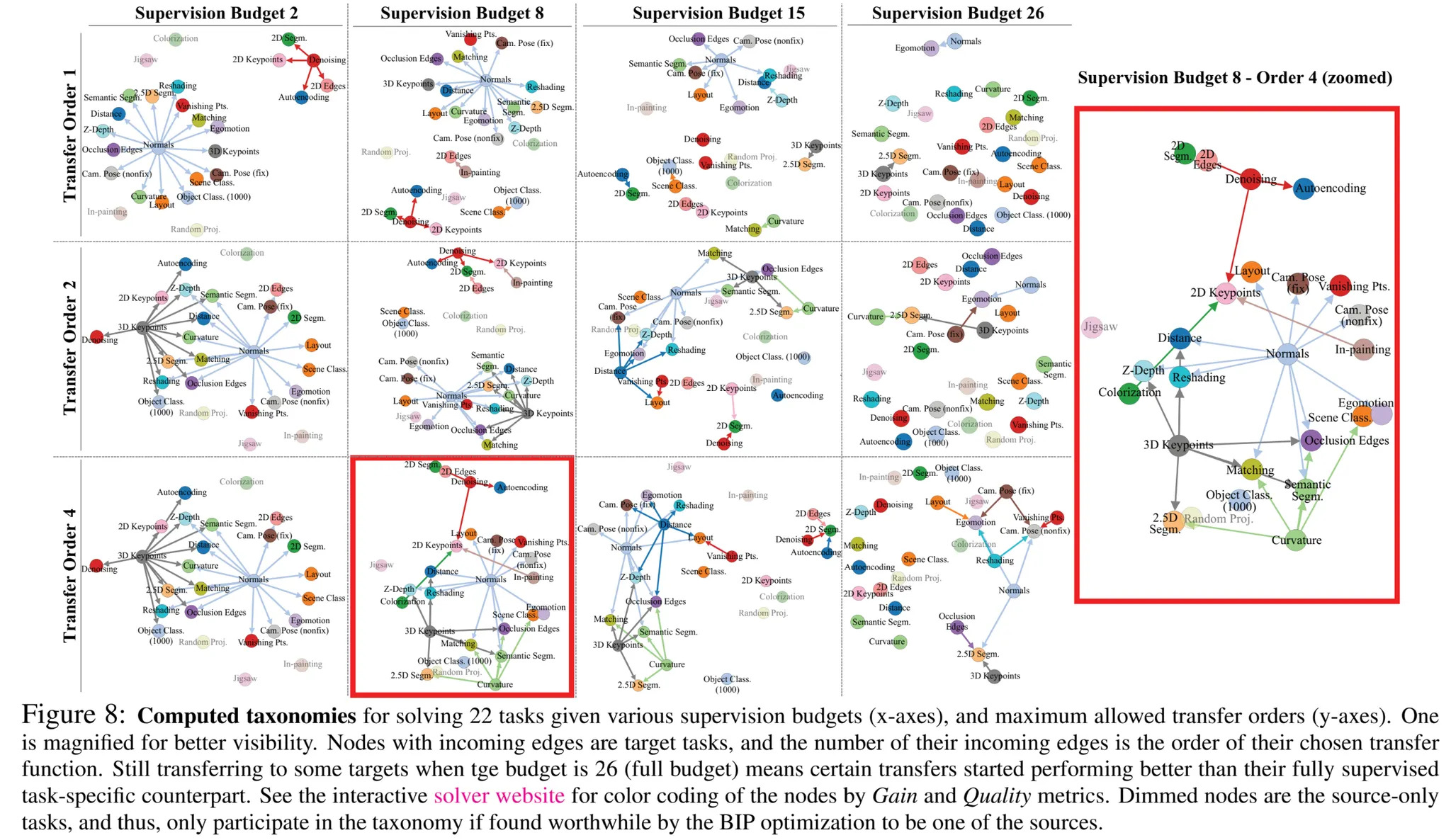
A global transfer policy which maximizes collective performance across all task
•
Formulated as subgraph selection where tasks are nodes and transfers are edge
Solve with Boolean Integer Programming (BIP)
Results
•
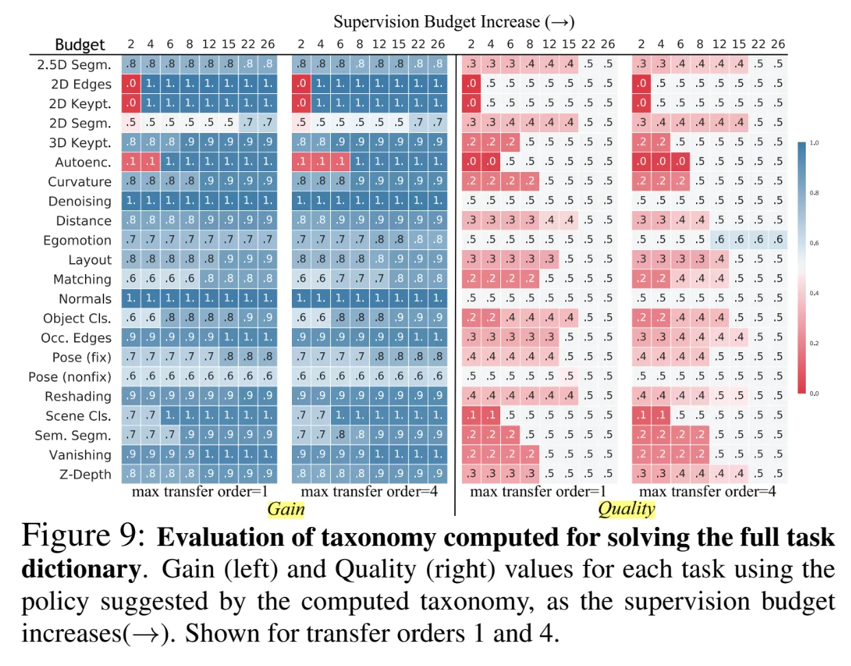
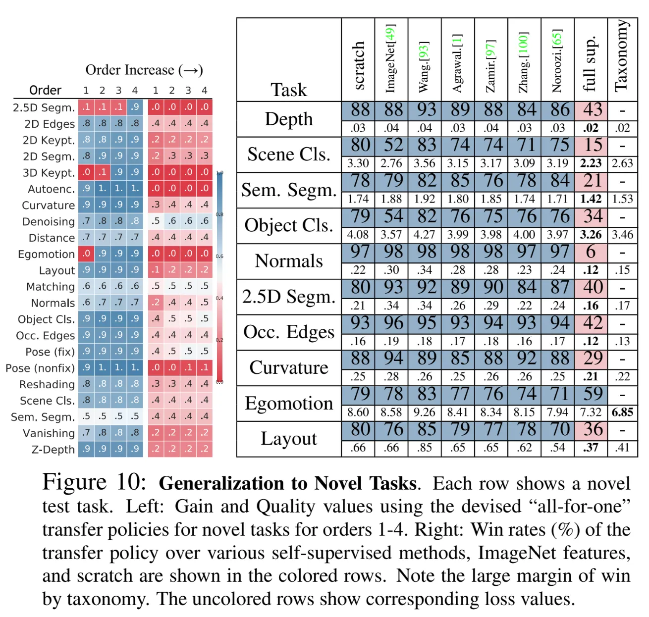
Evaluation metric : Win rate (%)→ 크면 클수록 좋다
: the proportion of test set images for which a baseline is beaten
•
Gain → lower bound 0.5
◦
win rate (%) against a network trained from scratch using the same training data as transfer networks. That is, the best that could be done if transfer learning was not utilized.
•
Quality → upper bound 0.5
◦
win rate (%) against a fully supervised network trained with 120k images (gold standard)
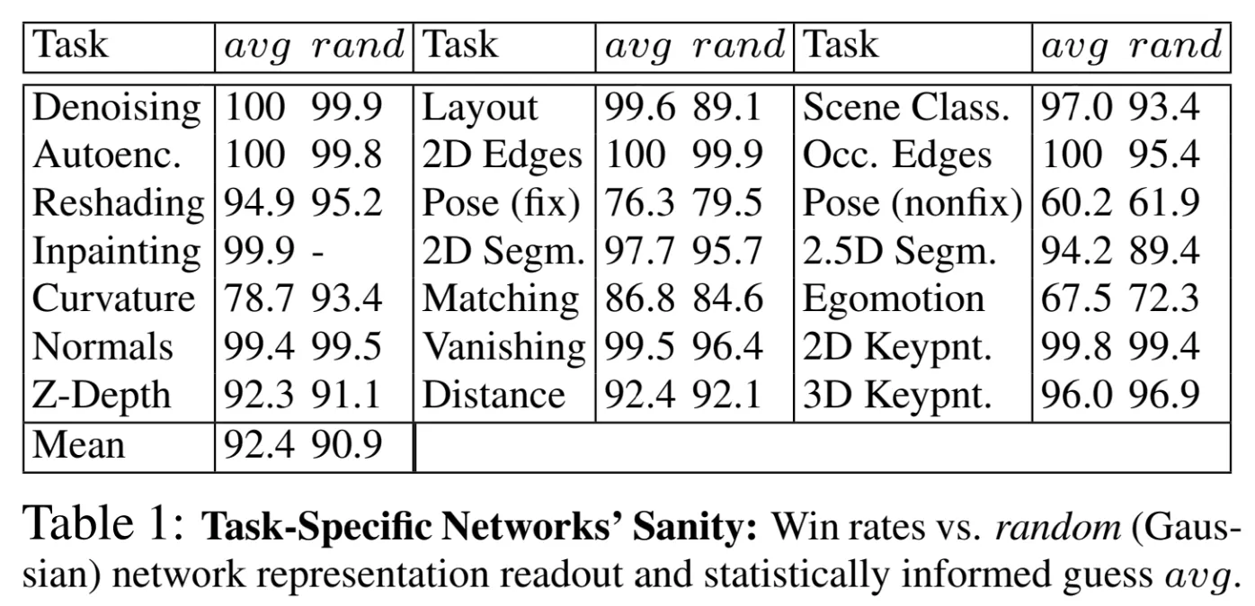
Sanity test (test-specific network가 얼마나 잘 학습되었는지)
Evaluation of computed taxonomies
Generalization to novel task
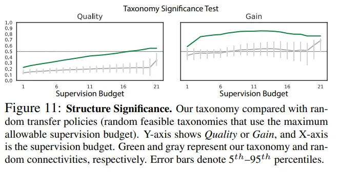
Significance test of the taxonomy structure
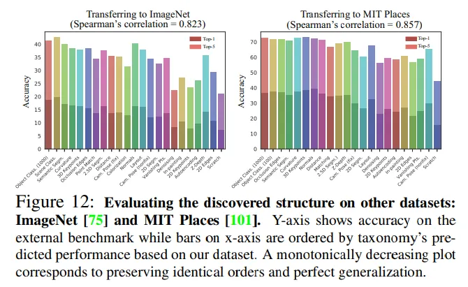
Evaluation on external dataset
•
Fine tuned our task-specific networks on other datasets (MIT Places for
scene classification, ImageNet for object classification)


